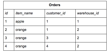
Complexity vs Simplicity: The LEFT OUTER JOIN vs the INNER JOINLet’s start with the basics – the Consider the following data with the corresponding query. |
Redshift’s JOIN clause is perhaps the second most important clause after SELECT clause, and it is used even more ubiquitously, considering how interconnected a typical application database’s tables are. Due to that connectivity between datasets, data developers require many joins to collect and process all the data points involved in most use cases. Unfortunately, as the number of tables you’re joining in grows, so does the sloth of your query. Those joins aren’t for nothing, either. A developer usually adds more joins because of their need for a more sophisticated result than a smaller (or perhaps more denormalized) dataset could yield. So how do we as data analysts, scientists, and engineers manage to balance complex queries against query time and just plain code readability? In this guide, we’ll discuss several tips for determining when and how to trade off simplicity for speed – or get the best of both worlds, when possible.
Complexity vs Simplicity: The LEFT OUTER JOIN vs the INNER JOIN
Let’s start with the basics – the LEFT OUTER JOIN vs. the INNER JOIN. These are probably the two most commonly used joins. Frequently, developers getting up to speed with writing SQL queries see that their left joins are producing “duplicate” results – so they change it out for an INNER JOIN.
Consider the following data with the corresponding query.
Tables
Query
SELECT c.state_residence, o.item_name, w.location
FROM customers c
LEFT OUTER JOIN orders o ON o.customer_id = c.id
LEFT OUTER JOIN warehouses w ON w.id = o.warehouse_id;
Results
(If you don’t believe me – check the appendix of this post. This query has been tested!)
You may believe that the duplicate final row is an error, and who cares about a row with mostly NULL values? This, dear reader, is a grave mistake. All left joins are valid – when joined on the right column and the correct select clause is given. My experience is that “duplicate” results spring from one of two sources – either a column that would differentiate the rows is missing (in this case, customers.first_name would do the trick) or there should be a GROUP BY clause in place. Often, the former solution would just serve to clutter the results, and in any case, I love GROUP BY – it forces you to think about what to DO with your “duplicate” rows. Is the count of records corresponding to the group valuable information? Is just the first record’s value sufficient to represent the group? Do you want to actually aggregate your group into a sum or mean? In our above case, grouping by all our select columns and adding a COUNT(*) column would provide insight into how many orders for a given state and item type were created.
There are many valid ways to group results, and they all demand you pay more rigorous attention to what you’re actually asking of your query. This can only be a good thing, as it gives you more clarity on what the real question is that you want to be answered. You might see now how replacing a left join with an inner join would’ve obscured the deeper insight, here; an inner join short-circuits the thinking behind two interesting results. First, we have multiple orders corresponding to the columns we’ve deemed important enough to select out. Second, there are some customers with no orders, and their state_residence is coming through in the results to elucidate that fact. If our business users are interested in tracking state-wide trends on orders, both of these facts are useful and would have been lost to an inner join.
Verdict: Higher complexity wins out almost every time, here – A LEFT OUTER JOIN producing “duplicate” results should be considered carefully by aggregating rows into groups with a deliberate aggregate function.


